Epsilon Theory will occasionally publish academic research of merit pertaining to financial and political markets.
You can read about our reasons and our guidelines here: Why Publish Academic Research?
If you have publishable academic research that you think expands our collective understanding of financial or political markets, and you’d like to give it access to our network of 100,000+ investment professionals, asset owners, academics and market enthusiasts, please send it to us at [email protected].
Will making academic journals irrelevant save the world? No.
But it’s a good start.
PDF Download: Quantile Tracking Errors (QuTE)
Authors
Mike Aguilar is a Teaching Associate Professor at the Department of Economics, University of North Carolina at Chapel Hill and the Chief Investment Officer at Cardinal Retirement Planning, Inc. in Durham, NC. Email: [email protected]
Ruyang Chengan is an Analyst at Dimensional Fund Advisors in Charlotte, NC. Email: [email protected]
Anessa Custovic is a Quantitative Research Analyst at Cardinal Retirement Planning, Inc in Durham, NC. Email: [email protected]
Abstract
The tracking error is a ubiquitous tool among active and passive portfolio managers, used widely for fund selection, risk management, and manager compensation. In this paper we show that traditional measures of tracking error are incapable of detecting variations in higher order moments (e.g. skewness and kurtosis). As a solution, we introduce a new class of Quantile Tracking Errors (QuTE), which measures differences in the quantiles of return distributions between a tracking portfolio and its benchmark. Through an extensive simulation study we show that QuTE can detect variations in higher order moments. We also offer guidance on the granularity of the quantile grid and weighting schemes for the relative importance of various quantiles. A case study illustrates the benefits of QuTE during the Dot Com Bubble and the Great Recession
INTRODUCTION
Traditional measures of tracking error are inadequate. Although there are several variants, most commonly tracking errors are cast as squared deviations between a tracking portfolio and benchmark over some period of time. However, this type of quadratic structure is inconsistent with the linear performance fees through which most managers are compensated (see Kritzman [16]). Instead, managers are incentivized to avoid extreme return deviations (Rudolf, Wolter, and Zimmermann [22]), which implies that higher order moments, such as kurtosis, are relevant. Moreover, Beasley, Meade and Chang [3] suggest that managers are incentivized to avoid consistently underperforming their benchmark, suggesting that skewness is also relevant.
Dorockov [8] and Blume and Edelen [5] point out that the goal of a tracking error is to measure how closely a portfolio can exactly replicate its associated benchmark. There is a preponderance of evidence that asset returns are non-Gaussian. Mills [18] documents excess skewness and kurtosis in daily asset returns, while Chung, Johnson and Schill [7] document it for monthly [1] asset returns as well. Therefore, tracking only the first two moments, as do conventional measures, is insufficient.
Other shortcomings of traditional tracking error measures have been cited. For instance, Pope, and Yadav [19] illustrate the bias in tracking error due to serial correlation in returns. Moreover, Ammann and Tobler [1] recognize that tracking error variance is subject to sampling error.
This paper makes two contributions to the literature on portfolio tracking. First, we detail a previously undocumented shortcoming of traditional tracking errors. Through a simulation study we show that traditional tracking errors (such as average tracking error and tracking error volatility) fail to detect situations in which the skewness (and/or kurtosis) of the tracking portfolio differs from that of the associated benchmark.
The second contribution of this paper is to introduce a class of quantile based tracking errors (QuTE). As we will discuss in Section 2.2, there are many variants of tracking error. Some have symmetric loss functions, structured via absolute or squared deviations. Meanwhile other variants incorporate asymmetries visa vis semi standard deviations, which are aligned with downside risk. Each have an analogue within our quantile based measures. We show that even the most basic of these QuTE measures is able to detect deviations in higher order moments of returns.
We begin with a detailed accounting of the traditional measures of tracking error alongside the newly proposed quantile based measures. We then conduct an extensive simulation study to explore the relative merits of QuTE. Finally, we document historical episodes where QuTE was able to detect important differences between a tracking portfolio and it’s benchmark, while the traditional measures were unresponsive.
Portfolio Tracking
In this section we detail the lineage of tracking errors and provide a compendium of its variants. We complement with an introduction of the new QuTE class of tracking errors.
Tracking Errors

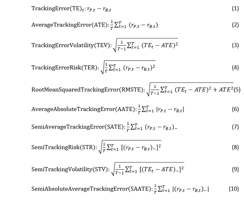

Equation (1) was seen first in the academic literature in Franks [10], which defined it simply “excess of benchmark returns”. Among practitioners, the object in Equation (1) is sometimes referred to as Tracking Difference.[2] Roll [20] refers to this object as “Tracking Error”, which we find to be commonly applied within the proceeding academic literature, and as such reserve that terminology throughout the balance of this paper. Note that the object in Equation (2) is simply an average of the Tracking Error over a period of time.
The object in Equation (3) is the next most commonly used variant of the term Tracking Error. Franks [10] refers to this object as Tracking Error, whereas Roll [20] refers to this as Tracking Error Volatility (TEV). Many proceeding academic studies (see Jorion [14]) use the TEV terminology. Moreover, Equation (3) is commonly referred to as Tracking Error among practitioners.[3] Often this is reported as an annualized value.[4] Equation (4) is subtly distinct, but is less often used in the literature than is Equation (3). Used by Ammann and Tobler [1], it captures the square root of the sum of the squared tracking error. Root Mean Squared Tracking Error (RMSTE) in Equation (5) was used by Chincarini and Kim [6] as a way to capture both the variability and the level of the tracking errors.
As noted by Kritzman [16], portfolio managers are rewarded by linear performance fees based upon the differences between their portfolio and the corresponding benchmark. Rudolf, Wolter and Zimmermann [22] argue, that due to this fact, linear deviations between the portfolio and benchmark give a more accurate description of the investors’ risk attitudes than do squared deviations. As such, tracking measures based off of absolute, rather than squared differences, such as those in Equation (6) and Equation (10) are sometimes advocated.
Both the quadratic and absolute measures heretofore are inconsistent with investor loss aversion. Rudolf, Wolter and Zimmermann [22] advocate the use of semi-variances for downside risk measurement. Equations (7) – (10) reflect this downside risk.
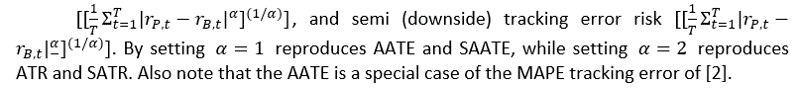
Finally, Beasley, Meade and Chang [3] introduce a generalized tracking error written as
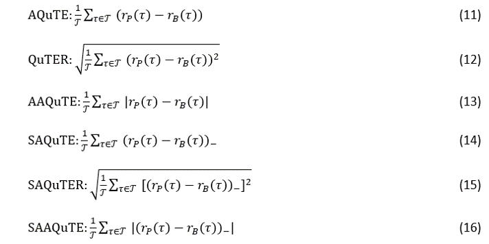
QuTE
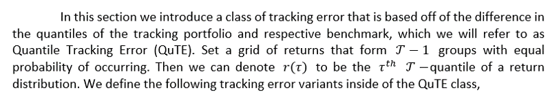
Intuitively, QuTE compares two assets via differences in the quantiles of their respective return distributions. This is especially useful in finance given the preponderance of returns with excess skew and kurtosis, and quantile-based methods’ ability to capture these distributions (see Rostek [21]). Moreover, a quantile based approach is consistent with the utility maximization via quantile maximization of Rostek [21], as well as with Giovannetti [12], who builds an asset pricing model consistent with CRRA preferences via quantile maximization.
Since the Value-at-Risk (VaR) is merely a quantile of a return distribution, we can see QuTE as matching on the space of VaR’s are various levels. Yamai and Yoshiba [24] show us that portfolio ranking via VaR is consistent with expected utility maximization and is free of tail risk. We adapt the findings of Rostek [21], who characterizes the behavior of an agent evaluating different (investment) alternatives by the -th quantile of the implied (return) distributions and selects the one with the highest quantile payoff. We can represent an investor’s preferences via the quantiles of the associated return distribution. In the context of benchmark tracking, we can then cast the investor’s preferences for deviations from their benchmark via the differences in the quantiles of the portfolio and benchmark. Portfolio construction with VaR based objective functions is increasingly common (see Gaivoronski and Pug [11] for recent examples). Moreover, a quantile based approach is especially attractive given the prevalence of VaR for portfolio risk management. For instance, Follmer and Leukert [9] uses VaR in the context of dynamic hedging.
Note that a natural analogue to QuTE is moment based matching, rather than quantile based. One could use a method of moments type estimator to match a select set of empirical moments between the benchmark and optimal portfolio. Although potentially attractive, a moment based approach lacks the flexibility of a nonparameteric quantile based method.
Notice the similarities with the tracking error measures defined in Section 2.1. Importantly, the averaging in the QuTE class is not done over time , but rather across quantile levels
. The QuTE measures never force the portfolio managers to compare his/her portfolio to the benchmark on a daily basis. This might mitigate the problem of “short termism” as indicated by Ma, Tang and Gomez [17]. Specifically, short evaluation periods for performance based compensation may damage fund performance by incentivizing managers to engage in such activities as risk shifting and window dressing to boost short-term performance.
Since there is a one-to-one mapping between the quantiles (returns) and the quantile levels (probabilities), portfolio tracking via QuTE can be cast within the wide literature of distribution matching. Cast this way, QuTER falls within the Fidelity Family of similarity measures. These types of measures are used in a wide variety of fields.
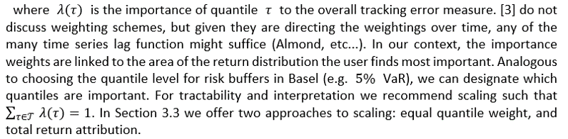
Beasley, Meade and Chang [3] expand their tracking error to accommodate for the case where someone might want to weigh the importance of the return deviations differently over time. Analogously, we introduce a quantile weighted version of QuTE. We illustrate below for the case of QuTER, but this approach can easily be extended to any of the measures within the QuTE family.

Simulation Study
In this section we explore the differences between QuTE and traditional TE tracking measures. Of particular importance, in subsection 3.1, is the sensitivity of each measure to differences in the empirical distributions of the benchmark and tracking portfolio. Subsections 3.2 and 3.3 focus on robustness of QuTE to various calibrations.
Sensitivity to Differences in Return Distributions
In this subsection we conduct a simulation study to evaluate the traditional tracking error measures of Section 2.1 as well as the QuTE based measures of Section 2.2. We craft a toy exercise that, while simple in nature, permits us to highlight the sensitivity of the tracking errors to differences in the underlying return distributions. Given the preponderance of evidence citing skewness and kurtosis (see Chung, Johnson and Schill [7], Mills [18], among others) in asset returns, coupled with the calls for linear performance measures a la Rudolf, Wolter and Zimmermann [22] and Kritzman [16], we consider deviations in these “higher order” moments.
We begin by creating a benchmark portfolio. For simplicity, we assume the returns of the benchmark follow a standard Normal distribution. We calibrate the length and empirical moments of the benchmark to match that of the monthly returns on Dow Jones Industrial Average over the period 1985 through 2019. This same index is used in a Case Study detailed in Section 4. Our simulations contain 10,000 paths, each of length 414 months.
Next, we generate a tracking portfolio that follows one of five distinct distributions, which are depicted in Table 1. In Case 0, the tracking portfolio has the same distribution as the benchmark portfolio. In Case 1, they differ only in the mean. Similarly, Case 2 varies in terms of variance, Case 3 in terms of skewness, and Case 4 in terms of kurtosis.[5]

We explore the ability of the various traditional tracking measures to detect differences in the mean (standard deviation, skewness, kurtosis) of the tracking portfolio and benchmark. As noted in Section 2.1, the TEV depicted in Equation (3) is the most commonly used tracking measure among academics and practitioners. We compare the TEV to ATE, TER, and RMSTE.[6]
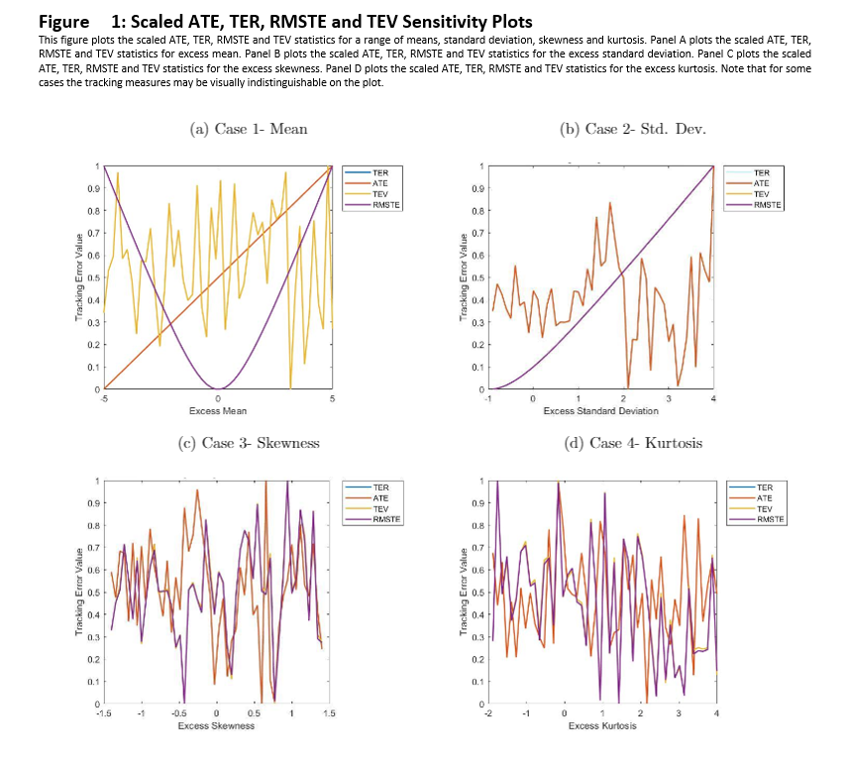
First, we vary the mean return of the tracking portfolio in excess of the benchmark (i.e. excess mean) in the range.[7] Next, we compute the ATE, TER, RMSTE and TEV for each of these values of excess mean, simulated and averaged over 10,000 paths. Finally, we scale [8] the values for each of the cases for ease of visual comparison. Panel A of Figure 1 depicts the ATE, TER, RMSTE and TEV values over the range of excess mean values. Panels B, C, and D similarly reflect excess standard deviation, skewness, and kurtosis.
A desirable measure of tracking error should achieve a minimum at an excess mean (standard deviation, skewness, kurtosis) of 0, i.e. when there is no difference between the tracking portfolio and benchmark, the tracking error measure should be at its low point. We find that ATE is unable to detect changes in any of the four moments. Meanwhile, TEV performs similarly to TER and RMSTE across Cases 2 through 4. In this sense, TEV is roughly equivalent to TER and RMSTE.
Next, we compare the traditional and quantile based tracking measures in terms of their abilities to detect differences in the underlying statistical distributions of the benchmark and tracking portfolios. Our comparison is centered around the TER of Equation (4) and the QuTER of Equation (12). We note our prior findings that TER is roughly equivalent to the popular TEV, which makes this comparison relevant. Moreover, we note that QuTER is a direct analogue of QuTER, providing a fair comparison.
In Table 2 we explore these relative sensitivities by computing the percent change in the (Qu)TER statistic relative to Case 0. The greater is the percent change in the (Qu)TER in Case 1 relative to Case 0, the more sensitive is that measure to variations in the means of the two series.

The p-value of 0 for Case 1 in Table 2 implies that the percent change in the QuTER statistic for Case 1 relative to Case 0 is not equal to the percent change in the TER statistic for Case 1 relative to Case 0. In fact, we find that QuTER and TER have unequal sensitivities to differences in each of the first four statistical moments. Moreover, one-tailed t-tests suggest that the QuTER is in fact more sensitive than TER in all Cases.
We explore these findings further by conducting a sensitivity analysis as we did above. Again, we vary the degree of mean returns in the tracking portfolio in excess of the benchmark (i.e. excess mean) in the range.[9] Next, we compute the TER and QuTER for each of these values of excess mean, simulated and averaged over 10,000 paths. Finally, we scale [10] the values for each of the cases for visual comparison. Panel A of Figure 2 depicts the TER and QuTER values over the range of excess mean values. Panels B, C, and D similarly reflect excess standard deviation, skewness, and kurtosis. Again, a desirable measure of tracking error should achieve a minimum at an excess mean (standard deviation, skewness, kurtosis) of 0, i.e. when there is no difference between the tracking portfolio and benchmark, the tracking error measure should be at its low point.
Panel A of Figure 2 suggests that TER and QuTER are both sensitive to variations in the mean return of the tracking portfolio and benchmark. They each reach minimum values near 0 excess mean, and rise at values above and below that amount. Similarly, Panel B illustrates that both TER and QuTER appear sensitive to deviations in excess standard deviation. However, Panels C and D illustrate that TER is not sensitive to deviations in skewness nor kurtosis. Meanwhile QuTER continues to respond to these excess variations. We note that these findings are consistent for ATE/AQuTE, AATE/AAQuTE, and ATR/AQuTER.


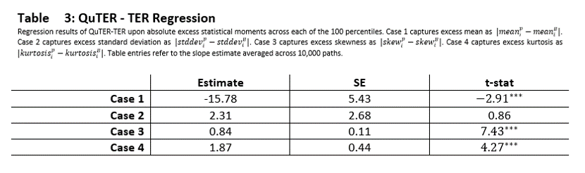
We can see from Table 3 that the estimated is positive and statistically significant for Cases 1, 3, and 4. This finding aligns with Figure 2, where QuTER appears to detect changes in the third and fourth moment, while TER is unable to do so. In terms of kurtosis, it appears that QuTER grows at least twice as fast per unit of change in excess kurtosis as TER does. Overall, we find that the sensitivities of the quantile based tracking errors are different, and in most cases larger, than the sensitivities of the traditional tracking errors.
Robustness to Granularity of Quantile Grid
In this subsection we explore whether the granularity of the quantile grid for the QuTE statistics impacts their ability to detect differences in the distributions of the tracking portfolio and the benchmark.
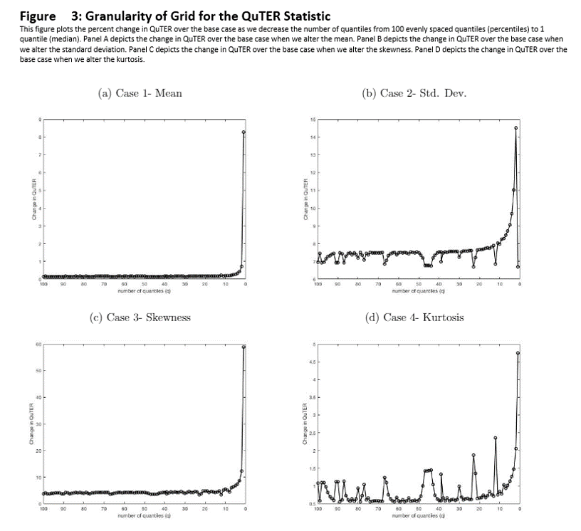
We repeat the exercise of Section 3.1 by simulating the benchmark returns as simple Gaussian noise and then varying the tracking portfolio in four ways; Case 1 alters the mean, Case 2 alters the variance, Case 3 alters the skewness, and Case 4 alters the kurtosis. Figure 3 depicts the percentage change in the QuTER statistic in a given Case relative to Case 0. The x-axis varies the size of the quantile grid (). The reported values are the median across 10,000 simulated paths.
We find that the percentage change in the QuTER statistic falls as the number of quantiles in the grid rises. The relationship appears to plateau near 10 quantiles. This stability is important, indicating that the QuTER measure is robust to choice of quantile grid.
Impact of Varying Quantile Weights
In this subsection we explore whether variations in the quantile weighting scheme impact QuTE’s ability to detect deviations between the distributions of the tracking portfolio and benchmark.
Blitz and Hottinga [4] illustrate how to compare various investment strategies via a Tracking Error framework. They consider weighting strategies by several methods of importance, such as tracking error, information ratio, and the like. In a similar vein, we can weight various quantiles by whatever criterion is most important to the investor. In the following, we consider four weighting schemes: equal weight, tail risk weight, down side risk weight, and total return attribution.
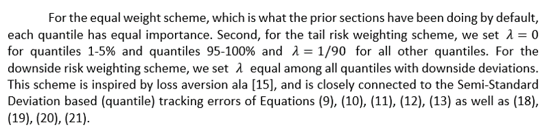
Finally, we consider a total return attribution weighting scheme, wherein each quantile is weighted according to its contribution to the portfolio’s total return. Specifically, using the equally spaced 100 quantile grid (i.e. percentiles), we compute the midpoint between each grid point to signify the average return in that return bin. We then compute the relative frequency of return observations that fall within that bin. Notice that the average return in each bin times the relative frequency of observations occurring within that bin is approximately equal to the total return. To compute the attribution of any given bin, we take the average bin return times relative frequency and divide by the total portfolio return.[11] By design these attributions sum to 1, and thus are viable choices for quantile weights .
In Figure 4 we illustrate how the QuTER objective function varies with the four aforementioned weighting schemes. Specifically, we repeat the exercise from Section 3.1 by simulating the tracking portfolio and benchmark. Each case varies one of the first four moments of the return distribution for the tracking portfolio. The height of each bar is the associated QuTER averaged over 10,000 paths. The number above each bar is the gross change of that average QuTER statistic relative to Case 0. For instance, the 1.1 above the first bar in Case 1 implies that the QuTER value for the equal weight scheme in Case 1 is 1.1 times as large as the equal weighting scheme QuTER statistic for Case 0. The legend can be read as follows: EW = Equal Weight, TR = Total Return Attribution, Tail = Tail Risk, and Down = Downside Risk.
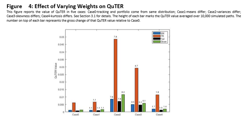
Within Case 1, we find that all of the weighting schemes are roughly equally (in)sensitive to excess mean returns. Gross changes are 1.1 for equal weighting, tail risk weighting, total return attribution, and for downside risk weighting. Within Case 2, total return and tail risk are again equally sensitive to variations in excess standard deviation, while downside is slightly more sensitive and equal weight is slightly less sensitive. For excess skewness, we find that tail risk is the most sensitive, downside is the least sensitive, while equal weight and total return have similar sensitivities. For excess kurtosis, equal weight and total return attribution are again similarly sensitive, with tail risk and downside risk being less so. In summary, a quantile weighting scheme of equal weight or total return attribution is robust to a wide array of differences in the underlying return distributions of the benchmark and tracking portfolio.[12]
Case Study
In this section we conduct two small case studies in order to illustrate the behavior of QuTE alongside a traditional measure of tracking error. The first case regards tracking the DJIA, while the second focuses on tracking the MSCI Emerging Markets index. We apply the QuTER and TER measures in both an unconditional and conditional setting.
Tracking the DJIA
In our first case study we use the Dow Jones Industrial Average (DJIA) as a benchmark and the DIA SPDR ETF as a tracking portfolio. The DJIA is a leading index of equity market returns in the U.S., being launched in May 26, 1896 and with approximately 1,876.70 dollars indexed to it’s performance. The DIA is among the largest of the DJIA ETF tracking portfolios, with an average of 7,102,449 USD in daily volume since the inception date. It is also one of the oldest ETFs to track the DJIA portfolio, with an inception date of January 13, 1998.

Our dataset contains monthly simple returns for both the DJIA (benchmark) and the DIA (tracking portfolio) over the period January 1998 to June 2019. Figure 5 depicts the time variation of the two return series overlayed upon one another. Simple visual inspection suggests they are quite similar. In fact, the correlation between the two return series is 0.99. Table 4 contains basic descriptive statistics such as mean, standard deviation, skewness, and kurtosis, as well as select quantiles of the two series. The last row contains the p-value for tests of equality between these various measures. A standard t-test is used for equal means. A standard F-test is used for equal variances. A two-way Kolmogorov-Smirnoff test is used to compare all of the four moments jointly. Finally, to compare the quantiles we use employ the Wilcox et al [23] test with a quantile estimator proposed by Harrell and Davis [13].

Figure 4 complements the comparisons in Table 4 by overlaying histograms of the tracking portfolio and benchmark in Panel A, and presenting a two-way QQ plot in Panel B. In addition, Table 5 presents various measures of (quantile) tracking errors. Note that the TE and QuTE values are not directly comparable given the different scaling of each measure.

Taken together, the above results reveal that the DIA has distributional properties that are remarkably similar to the DJIA, thereby supporting our visual inspection. Each of the moments and quantiles examined are statistically identical across the two portfolios.

Nonetheless, the two series can differ over time that are important to portfolio managers and investors. Figure 7 charts the difference in returns (TE) for each month. Deviations between the two series are particularly visible during the aftermath of the dot-com bubble in 2001 as well as during the Great Recession of 2008-2010. Of particular note is the variability in the TE over time. Figure 5 depicts the time variation in the difference in the first four moments of the tracking portfolio and benchmark. For the benchmark, we compute the mean return over a trailing three year window. We repeat for the tracking portfolio. Then we subtract those two values. That is a single point in Panel A of Figure 8. We then roll each sample forward by one month, recompute the means, and subtract. We continue that process for the rest of the times series, and repeat that exercise for the standard deviation (Panel B), skewness (Panel C), and kurtosis (Panel D).

In a similar fashion we compute the TER and QuTER statistics between the benchmark and tracking portfolio. Panel A of Figure 5 depicts the rolling tracking measures computed over rolling three year windows, while Panel B depicts the month to month percent change in each tracking measure.
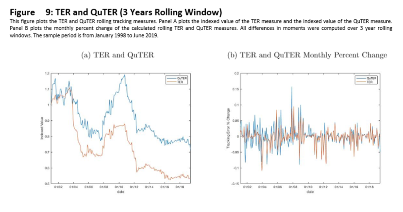
The statistical properties of the tracking portfolio differ from that of the benchmark over time. Our findings from Section 3 suggest that the QuTER statistic might be able to detect these differences when the TER cannot. For instance, as you can see from Figure 7, there is a large spike in the TE during 2001, followed by volatility of the TE until 2004. Figure 5 Panel A shows us that the differences in mean returns between DJIA and DIA was small and steady during this episode, while Panel D shows high differences in kurtosis. The TER is steady near 1.05 during this period, while the QuTER rises from 1 to 1.175, then falls back down to 1 by February 2004. These movements in the QuTER reflect its sensitivity to differences in return distributions that were not detected by TER.
Another episode of interest is the Great Recession. The TE swings wildly from 0.70 to 0.86 over the period 2008 to 2009. The mean return differences, as depicted in Panel A of Figure 5, vary between 0.17 and 0.20, and with it TER rises from 0.70 to 0.86. Notice that skewness changed from -0.01 to 0.11 and kurtosis from -0.05 to -0.10 over that period.[13] QuTER captured these movements, by increasing by almost 50 percent over that period, rising from 0.79 to almost 1.20, outpacing the roughly 22% change in TER.
Tracking the MSCI Emerging Markets Index
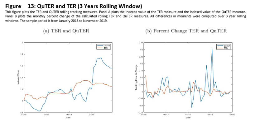
In our second case study we use the MSCI Emerging Markets Index (MSCI-EM) as a benchmark and the EEM iShares ETF as a tracking portfolio. We focus in on a recent episode that exemplifies the differences between TER and QuTER. Our dataset consists of monthly simple returns over the period January 2013 through November 2019.
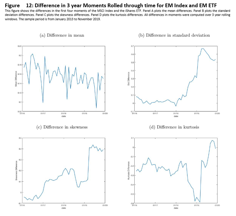
The correlation between the two return series is 0.97 during this sample period. As depicted in Figure 10 the empirical distributions are similar. Nonetheless, as depicted in Figure 11, there are differences between the two series. Analogous to Figure 5 in Section 4.1, Figure 5 illustrates the time variation in the differences of the first four empirical moments of the benchmark and tracking portfolio. Panels B, C, and D show stark time variation in the differences of standard deviation, skewness, and kurtosis.
TER is little changed during this period, as seen in Figure 5, ranging from approximately 1 to 1.3. Meanwhile, QuTER is able to detect these variations in the series, ranging between .8 and 1.7. The relative sensitivity of QuTER is even more stark in Panel B of Figure 5.

Conclusion
In this paper we document a shortcoming of traditional tracking error measures. Cast as a quadratic norm of return differences between a tracking portfolio and benchmark, traditional tracking error measures like TEV and TER are focused on only the first two moments of the underlying return distributions. As such, they are inconsistent with the manner with which most portfolio managers are compensated. If the portfolio and benchmark differ in ways other than the mean or variance, traditional measures are insufficient.
As a remedy, we introduce a new class of tracking errors that are based on the differences in the quantiles of the tracking portfolio and benchmark, namely QuTE. Just as there are myriad variants of tracking error, so too are there variants of QuTE (see Section 2 for a complete listing).
We show via simulation that a simple quadratic summary statistic (QuTER) is more sensitive to differences in higher order moments than is its TER counterpart. We also document in two cases studies situations wherein the QuTER statistic is able to detect important differences in tracking portfolios from their benchmarks, which the TER missed.
Our findings are directly relevant for ex-post performance measurement as well as risk evaluation. Differences in higher order moments matter, and quantile based measures of portfolio tracking provide a useful complement to traditional measures.
References
[1] Ammann, M. and Tobler, J. (2000). Measurement and decomposition of tracking error variance. Working paper, University of St. Fallen.
[2] Barro, D. and Canestrelli, E. (2009). Tracking error: a multistage portfolio model. Annals of Operations Research, 165(1):47-66.
[3] Beasley, J. E., Meade, N., and Chang, T. J. (2003). An evolutionary heuristic for the index tracking problem. European Journal of Operational Research, 148(3):621-643.
[4] Blitz, D. and Hottinga, J. (2001). Tracking error allocation. The Journal of Portfolio Management, 27.
[5] Blume, M. and Edelen, R. (2004). S&p 500 indexers, tracking error, and liquidity. The Journal of Portfolio Management, 30:37-46.
[6] Chincarini, L. and Kim, D. (2006). Quantitative Equity Portfolio Management An Active Approach to Portfolio Construction and Management: An Active Approach to Portfolio Construction and Management. McGraw- Hill.
[7] Chung, Y. P., Johnson, H., and Schill, M. J. (2006). Asset pricing when returns are non-normal: Famafrench factors versus higher order systematic comoments. The Journal of Business, 79(2):923-940.
[8] Dorockov, M. (2017). Comparison of etf’s performance related to the tracking error. Journal of International Studies, 10:154-165.
[9] Follmer, H. and Leukert, P. (1999). Quantile hedging. Finance and Stochastics, 3(3):251-273.
[10] Franks, E. C. (1992). Targeting excess-of-benchmark returns. The Journal of Portfolio Management, 18(4):6-12.
[11] Gaivoronski, A. and Pug, G. (2005). Value-at-Risk in Portfolio Optimization: Properties and Computational Approach. Journal of Risk, 7(2):1-31.
[12] Giovannetti, B. C. (2013). Asset pricing under quantile utility maximization. Review of Financial Economics, 22(4):169 – 179.
[13] Harrell, F. E. and Davis, C. E. (1982). A new distribution-free quantile estimator. Biometrika, 69(3):635-640.
[14] Jorion, P. (2004). Portfolio optimization with tracking-error constraints. Financial Analysts Journal, 59.
[15] Kahneman, D. and Tversky, A. (1979). Prospect theory: An analysis of decision under risk. Econometrica, 47(2):263-291.
[16] Kritzman, M. P. (1987). Incentive fees: Some problems and some solutions. FinancialAnalysts Journal, 43(1):21-26.
[17] Ma, L., Tang, Y., and Gomez, J. (2019). Portfolio manager compensation in the U.S. mutual fund industry. The Journal of Finance, 74(2):587-638.
[18] Mills, T. C. (1995). Modelling skewness and kurtosis in the london stock exchange ftse index return distributions. Journal of the Royal Statistical Society. Series D (The Statistician), 44(3):323-332.
[19] Pope, P. F. and Yadav, P. K. (1994). Discovering errors in tracking error. The Journal of Portfolio Management, 20(2):27-32.
[20] Roll, R. (1992). A mean/variance analysis of tracking error. The Journal of Portfolio Management, 18(4):13-22.
[21] Rostek, M. (2010). Quantile Maximization in Decision Theory*. The Review of Economic Studies, 77(1):339-371.
[22] Rudolf, M., Wolter, H.-J., and Zimmermann, H. (1999). A linear model for tracking error minimization. Journal of Banking & Finance, 23(1):85 – 103.
[23] Wilcox, R., Erceg-Hurn, D., Clark, F., and Carlson, M. (2014). Comparing two independent groups via the lower and upper quantiles. Journal of Statistical Computation and Simulation, N/A:9pp.
[24] Yamai, Y. and Yoshiba, T. (2002). On the validity of value-at-risk: Comparative analyses with expected shortfall. Monetary and Economic Studies, 20(1):57-85.
Notes
[1] [7] documents excess skewness and kurtosis for cross-sectional daily, weekly, monthly, quarterly and semi-annual asset returns.
[2] See for example, the ESMA https://www.esma.europa.eu/sites/default/files/library/2015/11/2012-832en_guidelines_on_etfs_and_other_ucits_issues.pdf, Morningstar https://media.morningstar.com/uk/MEDIA/Research_Paper/Morningstar_Report_Measuring_Tracking_Efficiency_in_ETFs_February_2013.pdf, and Vanguard https://www.vanguard.com.hk/documents/understanding-td-and-te-en.pdf
[3] CFA Institute https://www.cfainstitute.org/-/media/documents/support/programs/investment-foundations/19-performance-evaluation.ashx?la=en hash=F7FF3085AAFADE241B73403142AAE0BB1250B311, International Organization of Securities Commissions and European Securities and Markets Authority https://www.iosco.org/library/pubdocs/pdf/IOSCOPD414.pdf
[4] Zephyr https://www.styleadvisor.com/content/tracking-error, Vanguard https://www.vanguard.co.uk/documents/adv/literature/understand-excess.pdf, Envestnet https://www.envestnet.com/sites/default/files/documents/A%20Tracking%20Error%20Primer%20-%20White%20Paper.pdf
[5] Each series was simulated within Matlab using the pearsrnd function for a Pearson system of random numbers with moments calibrated to match the mean, standard deviation, skewness, and kurtosis of the monthly return of the Dow Jones Industrial Average over the period 1985 through 2019.
[6] The measures of absolute and semi tracking error are beyond the scope of this paper
[7] We also consider excess standard deviation in the range 0.10 to 5, excess skewness in the range -1.4 to 1.4, and excess kurtosis in the range 1 to 7.
[8] We scale as follows: Tracking Measure Value – min(Tracking Measure Value)/(max(Tracking Measure Value)-min(Tracking Error Value))
[9] We also consider excess standard deviation in the range 0.10 to 5, excess skewness in the range -1.4 to 1.4, and excess kurtosis in the range 1 to 7.
[10] We scale as follows: Tracking Measure Value – min(Tracking Measure Value)/(max(Tracking Measure Value)-min(Tracking Error Value))
[11] More precisely, we divide by the sum of the average bin returns times relative frequencies. Due to the averaging across the bins, this value may not be equal to the actual portfolio return in any given dataset, but will approach that value as the distance between the grid points approach 0.
[12] Our findings are similar for AQuTE and AAQuTE
[13] During this time period, the difference in kurtosis reached a high of -0.50.
PDF Download: Quantile Tracking Errors (QuTE)


Start the discussion at the Epsilon Theory Forum